class: center, middle, inverse, title-slide # Geospatial data in R ### Ian Hough ### 2019-10-17 - R in Grenoble --- # Overview #### Data manipulation * Vector data: [sf](https://r-spatial.github.io/sf/) * Raster data: [raster](https://github.com/rspatial/raster) #### Visualization * Thematic maps: [tmap](https://github.com/mtennekes/tmap) * Raster data: [rasterVis](https://oscarperpinan.github.io/rastervis/) * Interactive maps: [tmap](https://github.com/mtennekes/tmap) & [mapview](https://r-spatial.github.io/mapview/) #### Resources * [Lovelace et al. (2019): Geocomputation with R](https://geocompr.robinlovelace.net/index.html) * [Pebesma & Bivand (forthcoming): Spatial Data Science](https://keen-swartz-3146c4.netlify.com) * [Bivand et al. (2013): Applied Spatial Data Analysis with R](https://www.springer.com/gp/book/9781461476177) * [RSpatial.org](https://rspatial.org) * [r-spatial.org](https://www.r-spatial.org) * [CRAN Task View: Analysis of Spatial Data](https://cran.r-project.org/web/views/Spatial.html) * [r-sig-geo mailing list](https://stat.ethz.ch/mailman/listinfo/R-SIG-Geo/) --- # Why use R for geospatial data? * Automation + reproducibility (vs. ArcGIS, QGIS, etc.) * Ease of use (vs. C++/Java) * Rich ecosystem of tools for statistical analysis (spatial + not), predictive modeling, and visualisation (vs. Python) --- # Geospatial data models .pull-left[ ### Vector 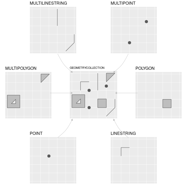 ] .pull-right[ ### Raster 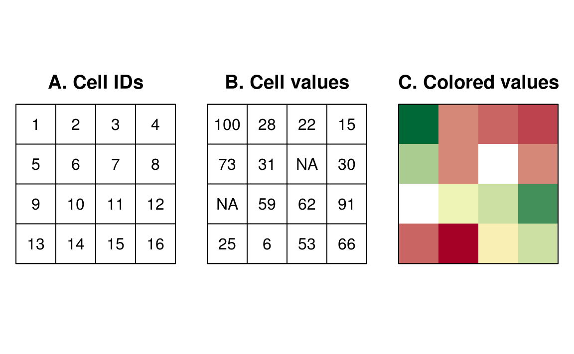 ] .footnote[*Img: Lovelace et al. 2019*<sub>] --- # sf package "Simple features" = OGC standard for representation of vector spatial data, used by many spatial libraries (GDAL, GEOS), databases (PostGIS), etc. Extends `data.frame` or `tibble` by adding a geometry column. This makes it easy to work with sf object as you would any other data.frame (pipe-based workflows, dplyr, etc.) Provides consistent interface to [gdal](https://gdal.org) and [geos](https://trac.osgeo.org/geos) libraries. Largely supersedes [sp](https://cran.r-project.org/web/packages/sp/index.html), `rgdal`, and `rgeos` packages (although some other packages have not yet been updated to work with sf). --- # sf setup #### Prerequisites ```r install.packages("sf") install.packages("spData") # for demo datasets install.packages("tidyverse") # to demonstrate tidyverse compatibility ``` *Note:* the R spatial ecosystem depends on three open-source C/C++ libraries: * [gdal](https://gdal.org): translator for geospatial data formats * [geos](https://trac.osgeo.org/geos): spatial geometry engine * [proj](https://proj.org): coordinate reference system transformations These are included with the *binary* release of [sf](https://r-spatial.github.io/sf/) for Windows and Mac. If you use Unix or install packages from source you will need to install these separately. --- # sf example ```r library(sf) ``` ``` ## Linking to GEOS 3.6.1, GDAL 2.2.3, PROJ 4.9.3 ``` ```r library(spData) # demo datasets ``` ``` ## To access larger datasets in this package, install the spDataLarge ## package with: `install.packages('spDataLarge', ## repos='https://nowosad.github.io/drat/', type='source')` ``` ```r library(tidyverse) # show compatibility with tidyverse ``` ``` ## -- Attaching packages ---------------------------------------------------- tidyverse 1.2.1 -- ``` ``` ## v ggplot2 3.2.1 v purrr 0.3.2 ## v tibble 2.1.3 v dplyr 0.8.3 ## v tidyr 1.0.0 v stringr 1.4.0 ## v readr 1.3.1 v forcats 0.4.0 ``` ``` ## -- Conflicts ------------------------------------------------------- tidyverse_conflicts() -- ## x dplyr::filter() masks stats::filter() ## x dplyr::lag() masks stats::lag() ``` ```r class(world) ``` ``` ## [1] "sf" "tbl_df" "tbl" "data.frame" ``` ```r names(world) ``` ``` ## [1] "iso_a2" "name_long" "continent" "region_un" "subregion" ## [6] "type" "area_km2" "pop" "lifeExp" "gdpPercap" ## [11] "geom" ``` --- # sf geometry column is sticky ```r # Sticky geometry column world[1:3, 2] ``` ``` ## Simple feature collection with 3 features and 1 field ## geometry type: MULTIPOLYGON ## dimension: XY ## bbox: xmin: -180 ymin: -18.28799 xmax: 180 ymax: 27.65643 ## epsg (SRID): 4326 ## proj4string: +proj=longlat +datum=WGS84 +no_defs ## # A tibble: 3 x 2 ## name_long geom ## <chr> <MULTIPOLYGON [°]> ## 1 Fiji (((180 -16.06713, 180 -16.55522, 179.3641 -16.80135, 178.7~ ## 2 Tanzania (((33.90371 -0.95, 34.07262 -1.05982, 37.69869 -3.09699, 3~ ## 3 Western Saha~ (((-8.66559 27.65643, -8.665124 27.58948, -8.6844 27.39574~ ``` ```r # Get a single column world$iso_a2 %>% head ``` ``` ## [1] "FJ" "TZ" "EH" "CA" "US" "KZ" ``` --- # sf pipe-based workflow ```r world %>% dplyr::filter(continent == "Africa") %>% dplyr::select(pop) %>% plot(main = "Population") ``` 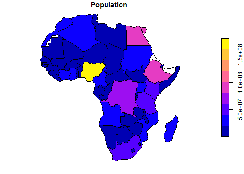<!-- --> --- # sf functions All sf functions start with a `st_` prefix (for "spatial-temporal", taken from PostGIS). Reading / writing - works with files or databases ```r st_read() st_write() ``` Inspection ```r st_bbox() # bounding box st_coordinates() st_crs() st_geometry() # get the geometry column ``` To / from sp ```r world_sp <- as(world, "Spatial") world_sf <- st_as_sf(world_sp) ``` --- # sf to / from data.frame ```r # sf to data.frame world_df <- st_drop_geometry(world) # data.frame to sfc set.seed(1) pts <- data.frame(lat = runif(5, 30, 80), lon = runif(5, -5, 10)) %>% st_as_sf(coords = c("lon", "lat"), crs = 4326) # EPSG:4326 = WGS84 plot(world$geom) plot(pts, pch = 19, cex = 2, col = "blue", add = T) ``` 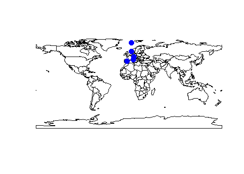<!-- --> --- # sf coordinate reference systems ```r # Get CRS st_crs(world) ``` ``` ## Coordinate Reference System: ## EPSG: 4326 ## proj4string: "+proj=longlat +datum=WGS84 +no_defs" ``` ```r # Project using EPSG code st_transform(world, crs = 3035) %>% st_crs() ``` ``` ## Coordinate Reference System: ## EPSG: 3035 ## proj4string: "+proj=laea +lat_0=52 +lon_0=10 +x_0=4321000 +y_0=3210000 +ellps=GRS80 +towgs84=0,0,0,0,0,0,0 +units=m +no_defs" ``` ```r # Project using proj4string st_transform(world, crs = "+proj=sinu +lon_0=0 +x_0=0 +y_0=0 +a=6371007.181 +b=6371007.181 +units=m +no_defs") %>% st_crs() ``` ``` ## Coordinate Reference System: ## No EPSG code ## proj4string: "+proj=sinu +lon_0=0 +x_0=0 +y_0=0 +a=6371007.181 +b=6371007.181 +units=m +no_defs" ``` --- # Simple spatial subsetting ```r world[pts, "iso_a2"] ``` ``` ## although coordinates are longitude/latitude, st_intersects assumes that they are planar ``` ``` ## Simple feature collection with 2 features and 1 field ## geometry type: MULTIPOLYGON ## dimension: XY ## bbox: xmin: -9.392884 ymin: 35.94685 xmax: 15.017 ymax: 54.9831 ## epsg (SRID): 4326 ## proj4string: +proj=longlat +datum=WGS84 +no_defs ## # A tibble: 2 x 2 ## iso_a2 geom ## <chr> <MULTIPOLYGON [°]> ## 1 DE (((14.11969 53.75703, 14.35332 53.24817, 14.07452 52.98126, 14.43~ ## 2 ES (((-7.453726 37.09779, -7.537105 37.4289, -7.166508 37.80389, -7.~ ``` --- # sf quantities and geometric operations ```r st_area() st_buffer() st_contains() st_difference() st_intersects() st_intersection() st_length() st_overlaps() st_touches() st_union() ... ``` --- ### sf and ggplot2 ```r library(ggplot2) ggplot() + geom_sf(data = world, aes(fill = iso_a2), show.legend = FALSE) + geom_sf(data = pts) + coord_sf(crs = "+proj=robin +lon_0=0 +x_0=0 +y_0=0 +datum=WGS84 +units=m +no_defs") ``` 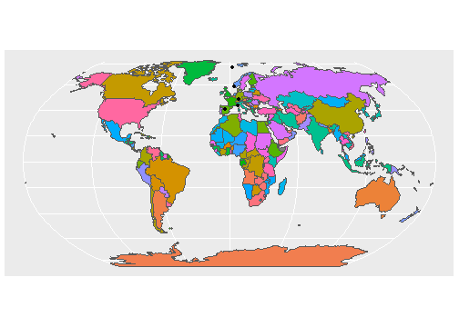<!-- --> --- # raster package Three types of raster objects * `RasterLayer` = a single layer (e.g. elevation) * `RaterStack` = multiple layers with the same spatial extent and CRS (e.g. daily temperature); more flexible than RasterBrick (layers can be mix of in memory and multiple files) * `RasterBrick` = like a RasterStack but all layers are contained in a single file; faster processing compared to RasterStack A key feature of the raster package is that it only loads data into memory when needed. If there is insufficient memory and the `filename` argument is provided, raster functions will process data in chunks and write directly to disk rather than loading into memory. Note: `raster` relies on `sp` and `rgdal`. The new [stars](https://r-spatial.github.io/stars/) package is intended to supersede `raster` and will provide a structure and interface more similar to `sf` and support for multidimensional data cubes (e.g. x, y, z, time). --- # raster setup ```r install.packages("sp") # imported by raster install.packages("rgdal") # needed for reading/writing many data formats install.packages("raster") ``` ```r library(raster) ``` ``` ## Loading required package: sp ``` ``` ## ## Attaching package: 'raster' ``` ``` ## The following object is masked from 'package:dplyr': ## ## select ``` ``` ## The following object is masked from 'package:tidyr': ## ## extract ``` Watch out for masking of `dplyr::select` and `tidyr::extract`! --- # raster example ```r t2m <- raster::brick("data/era5_t2m.tif") raster::inMemory(t2m) ``` ``` ## [1] FALSE ``` ```r t2m ``` ``` ## class : RasterBrick ## dimensions : 37, 55, 2035, 24 (nrow, ncol, ncell, nlayers) ## resolution : 0.25, 0.25 (x, y) ## extent : -5.375, 8.375, 42.125, 51.375 (xmin, xmax, ymin, ymax) ## crs : +proj=longlat +datum=WGS84 +no_defs +ellps=WGS84 +towgs84=0,0,0 ## source : C:/Users/Ian/code/2019-10_r-in-grenoble_geospatial/data/era5_t2m.tif ## names : era5_t2m.1, era5_t2m.2, era5_t2m.3, era5_t2m.4, era5_t2m.5, era5_t2m.6, era5_t2m.7, era5_t2m.8, era5_t2m.9, era5_t2m.10, era5_t2m.11, era5_t2m.12, era5_t2m.13, era5_t2m.14, era5_t2m.15, ... ## min values : 275.0910, 274.7592, 274.4634, 274.3012, 274.0129, 275.2710, 276.0705, 277.9212, 280.0212, 281.6605, 282.2485, 283.1449, 283.8315, 283.6270, 282.9048, ... ## max values : 293.2530, 293.2009, 293.1298, 293.0960, 293.0639, 293.0323, 293.0066, 294.9174, 296.0506, 297.1310, 297.9987, 298.8321, 299.9331, 300.5916, 300.6237, ... ``` --- ```r names(t2m) <- paste0("t2m_20180601_", 0:23) # Get one or more layers t2m[[1:3]] %>% plot ``` 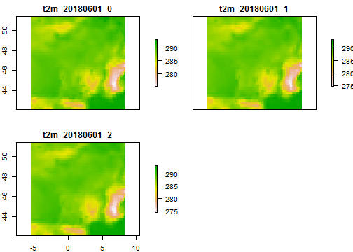<!-- --> --- ```r # Get values from a single layer t2m$t2m_20180601_0[1:3, 1:3] ``` ``` ## [1] 286.7862 286.3626 286.6148 287.4074 287.1633 287.4659 287.7788 287.6613 ## [9] 287.6613 ``` ```r # Cells are indexed from the top left corner along rows then by columns raster::xyFromCell(t2m, c(1, 55, 56)) ``` ``` ## x y ## [1,] -5.25 51.25 ## [2,] 8.25 51.25 ## [3,] -5.25 51.00 ``` --- # raster functions Reading / writing ```r raster::raster() # create or read a RasterLayer raster::stack() # create or read a RasterStack raster::brick() # create or read a RasterBrick raster::writeRaster() # save to disk ``` Inspection ```r raster::crs() # get or set CRS raster::projection() # get or set CRS raster::coordinates() raster::extent() # bounding box ``` --- # Projection ```r # Uses bilinear or nearest neighbour t2m$t2m_20180601_0 %>% projectRaster(crs = "+proj=laea +lat_0=52 +lon_0=10 +x_0=4321000 +y_0=3210000 +ellps=GRS80 +towgs84=0,0,0,0,0,0,0 +units=m +no_defs") %>% plot ``` 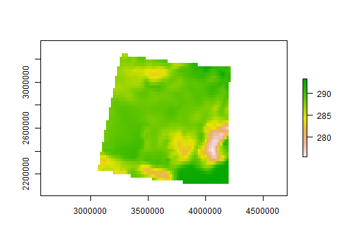<!-- --> ```r raster::projectRaster()crs() # get or set CRS raster::projection() # get or set CRS raster::coordinates() raster::extent() # bounding box ``` --- # raster -> vector ```r raster::rasterToPoints() # returns centroids raster::rasterToPolygons() # returns borders ``` ```r plot(rasterToPoints(t2m$t2m_20180601_0)) plot(world$geom, add = T) ``` 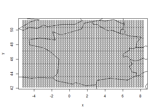<!-- --> --- # vector -> raster ```r france <- world[, "iso_a2"] %>% dplyr::filter(iso_a2 == "FR") %>% st_cast("POLYGON") %>% mutate(area = st_area(geom)) %>% dplyr::arrange(-area) %>% .[1, ] ``` ``` ## Warning in st_cast.sf(., "POLYGON"): repeating attributes for all sub- ## geometries for which they may not be constant ``` ```r fr_rst <- raster::rasterize(france, t2m) plot(fr_rst, axes = FALSE, box = FALSE) ``` 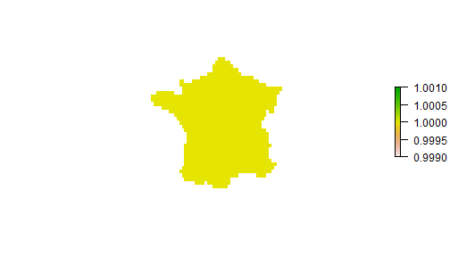<!-- --> --- # raster operations ```r raster::area() # area of each cell raster::crop() # reduce extent by that of a raster a spatial object raster::extract() # get values at locations of points or polygons raster::focal() # moving window summaries raster::zonal() # zonal statistics based on "zones" defined by layers of a raster value ... ``` --- # Map algebra ```r plot(max(t2m) * fr_rst) ``` 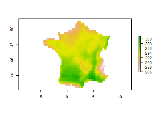<!-- --> --- # Mapping Livecoding: [mapping_demo.R](https://github.com/ihough/talk_2019-10_geospatial_r-in-grenoble/blob/master/mapping_demo.R)